Methods

This page states every statistic MedAgentRx computes, its assumptions and its source. All arithmetic is in float64. Every random step takes an explicit seed. A statistic that cannot be computed raises an error; it never returns NaN.

Notation: m positives and n negatives on the locked test set; alpha_k is the one-sided level available to update k.

AUROC and the paired DeLong test

The AUROC and the covariance of several AUROCs on the same rows follow DeLong, DeLong and Clarke-Pearson (1988). They are computed with the midrank algorithm of Sun and Xu (2014), which runs in O(n log n). Tied scores count one half. Variances use n - 1 denominators, matching the R package pROC.

Non-inferiority of a new model against a reference with margin delta:

• H0: AUC_new - AUC_ref <= -delta.
• Statistic: z = (estimate + delta) / SE, where SE comes from the paired covariance.
• H0 is rejected when z exceeds the 1 - alpha_k quantile of a Student t distribution with min(positives, negatives) - 1 degrees of freedom.
• The report gives the one-sided p-value and the two-sided (1 - 2 alpha_k) interval with the same critical value. Its lower bound exceeds -delta exactly when H0 is rejected.

Small-sample reference. The normal reference is the usual large-sample form of the DeLong test. In the validation grid it gave a type I error of 0.060 with 25 positives, at the edge of the accepted band. The t reference brings this to 0.054 and differs from the normal quantile only in the third decimal once there are hundreds of events. The statistic, its standard error and the agreement with pROC are unchanged.

At least two positives and two negatives are needed for a variance. Subgroup intervals use the same t reference with each subgroup's own degrees of freedom.

Validation. On four fixed datasets, including one with heavy ties, the AUC agrees with pROC 1.19 (roc.test(method = "delong", paired = TRUE)) within 1e-8, and the standard errors and z within 1e-6. CI recomputes the pROC values on every run.

Paired stratified bootstrap

Positives and negatives are resampled separately with replacement, so each replicate keeps the observed class counts. Both models are evaluated on the same resampled rows. The default is B = 2000 replicates.

Two intervals are reported:

• Percentile: the alpha / 2 and 1 - alpha / 2 quantiles of the replicates.
• BCa (Efron 1987): the bias correction z0 comes from the share of replicates below the estimate. The acceleration comes from a grouped jackknife: each class is split into up to 200 groups, and one group is left out at a time. With one row per group this is the ordinary jackknife. Grouping keeps the cost bounded on large test sets.

The bootstrap is used for net benefit, ECE and AUPRC, for sparse sensitivity and specificity comparisons, and as a cross-check on DeLong.

Sensitivity and specificity at the operating threshold

A row is predicted positive when its risk is at least the threshold. Within the relevant class, n10 counts rows correct only under the new model and n01 rows correct only under the reference. The difference is (n10 - n01) / n.

The interval is the score interval of Tango (1998), solved by bisection with the restricted maximum likelihood estimate of the discordant cell. When fewer than 10 pairs are discordant, the paired stratified bootstrap percentile interval is used instead. The criterion passes when the lower bound of the (1 - 2 alpha_k) interval exceeds -margin.

Calibration

• Slope: b from the logistic recalibration logit(P(y = 1)) = a + b * logit(p).
• Calibration-in-the-large: a from the offset model logit(P(y = 1)) = a + logit(p), slope fixed at 1.
• Both models are fitted by Newton-Raphson with step halving.
• Probabilities are clipped to [1e-10, 1 - 1e-10] before the logit.
• If risk perfectly separates the outcomes, the slope is not estimable and an error is raised.
• Brier score: the mean of (p - y)^2.
• ECE: the weighted mean absolute gap between observed and predicted risk over 10 equal-mass bins.
• Calibration curve: equal-mass bins for points, and a pool-adjacent-violators isotonic fit for the smooth curve.

Net benefit

Decision curve analysis of Vickers and Elkin (2006):

NB(t) = TP / n_total - FP / n_total * t / (1 - t)

It is evaluated at each plan threshold t. The difference between models has a paired bootstrap interval. Treat-all is prevalence - (1 - prevalence) * t / (1 - t).

Subgroups and multiplicity

For each subgroup level, the AUROC difference is tested for non-inferiority with margin max_drop. The update passes only if every subgroup is non-inferior. That is an intersection-union test (Berger 1982): each subgroup may be tested at the full level, and the chance of wrongly passing an update that harms some subgroup stays at most alpha. This is multiplicity: none, the default in init and the example.

Holm or Bonferroni would also bound the chance of wrongly calling any single subgroup non-inferior. The pass or fail decision on the whole update does not need that, and it makes passing harder. Both remain as stricter options:

• holm: the Holm (1979) step-down procedure. Each hypothesis is tested, and its interval reported, at the level it reached in the step-down sequence. Hypotheses after the first failure are reported at the level of that failure.
• bonferroni: every subgroup is tested at alpha divided by the number of subgroups.

A subgroup with fewer than min_events positives or negatives is reported as insufficient evidence.

Error control across updates

• Bonferroni: alpha_k = alpha_total / max_updates. This controls the family-wise error rate over the life of the plan.
• Alpha-investing (Foster and Stine 2008):
• Initial wealth is W0 = alpha_total * (1 - alpha_total).
• Update k tests at (W / (1 + W)) / R, where R is the number of updates still allowed.
• Showing non-inferiority earns alpha_total. Failing costs alpha_k / (1 - alpha_k).
• This controls the marginal false discovery rate, not the family-wise error rate.

The ledger records the level used by every evaluation, including failed ones.

Bio-creep guard

Every update is tested against the previous version and against the anchor. The lower bound of the interval for AUC_new - AUC_anchor must stay at or above -max_drop_vs_anchor. This stops a chain of individually non-inferior updates from drifting downwards (Feng et al. 2021).

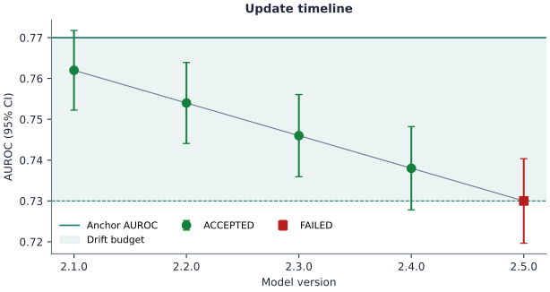
In the demo, five updates each lose 0.008 AUROC. Each is non-inferior to the one before, but the fifth exceeds the plan's drift budget against the authorised version and fails.

Power

The variance of one AUROC follows Hanley and McNeil (1982):

V = [A(1 - A) + (m - 1)(Q1 - A^2) + (n - 1)(Q2 - A^2)] / (m n)
Q1 = A / (2 - A)
Q2 = 2 A^2 / (1 + A)

For two models with the same expected AUROC and correlation r between the estimates, the paired difference has variance 2 V (1 - r). Power at true difference d is Phi((d + margin) / SE - z(1 - alpha)). A small simulation with binormal scores confirms the approximation.

medagentrx sample-size inverts this formula. It finds, by bisection, the smallest test set whose power reaches the target, with positives set by the expected prevalence. Given a plan, it takes the smallest AUROC margin, the level of the first update under the plan's alpha spending and the plan's minimum power. For example, AUROC 0.80, prevalence 0.12, margin 0.02, level 0.05 / 12 and correlation 0.6 need 15,088 rows for 80 percent power. The correlation of the two AUROC estimates matters most. Retraining the same architecture on more data usually gives 0.5 to 0.8, and higher correlation needs fewer rows. Estimate it from an earlier pair of versions when you can.

Population shift

• Numeric features: standardised mean difference (mean_1 - mean_2) / sqrt((s_1^2 + s_2^2) / 2).
• Categorical features: the multivariate definition of Yang and Dalton (2012), over level proportions without the first level.
• An absolute value above 0.1 gives a warning.

References

• DeLong E.R., DeLong D.M., Clarke-Pearson D.L. Comparing the areas under two or more correlated receiver operating characteristic curves: a nonparametric approach. Biometrics 1988;44:837 to 845.
• Sun X., Xu W. Fast implementation of DeLong's algorithm for comparing the areas under correlated receiver operating characteristic curves. IEEE Signal Processing Letters 2014;21:1389 to 1393.
• Efron B. Better bootstrap confidence intervals. Journal of the American Statistical Association 1987;82:171 to 185.
• Tango T. Equivalence test and confidence interval for the difference in proportions for the paired-sample design. Statistics in Medicine 1998;17:891 to 908.
• Vickers A.J., Elkin E.B. Decision curve analysis: a novel method for evaluating prediction models. Medical Decision Making 2006;26:565 to 574.
• Holm S. A simple sequentially rejective multiple test procedure. Scandinavian Journal of Statistics 1979;6:65 to 70.
• Foster D.P., Stine R.A. Alpha-investing: a procedure for sequential control of expected false discoveries. Journal of the Royal Statistical Society B 2008;70:429 to 444.
• Feng J., Emerson S., Simon N. Approval policies for modifications to machine learning-based software as a medical device: a study of bio-creep. Biometrics 2021;77:31 to 44.
• Hanley J.A., McNeil B.J. The meaning and use of the area under a receiver operating characteristic (ROC) curve. Radiology 1982;143:29 to 36.
• Yang D., Dalton J.E. A unified approach to measuring the effect size between two groups using SAS. SAS Global Forum 2012, paper 335.
• Robin X. et al. pROC: an open-source package for R and S+ to analyze and compare ROC curves. BMC Bioinformatics 2011;12:77.